Binomial Finance
Here's an HTML rendition explaining binomial finance in about 500 words:
Binomial Option Pricing Model
The Binomial Option Pricing Model (BOPM) is a popular method for valuing options. Unlike the Black-Scholes model, which relies on a continuous-time stochastic process, the BOPM uses a discrete-time model, making it conceptually simpler and more versatile. It's particularly useful for valuing options with complex features or when underlying asset returns don't perfectly fit a log-normal distribution.
Core Concepts
The model works by constructing a binomial tree representing the possible paths of the underlying asset's price over the option's life. At each node in the tree, the price can either go "up" or "down" by a certain factor. These factors are determined by volatility and time to expiration. The key is to create a risk-free portfolio at each node, comprising the option and the underlying asset, that guarantees the same payoff regardless of whether the price goes up or down.
The model rests on a few key assumptions:
- The price of the underlying asset follows a binomial distribution.
- There are only two possible prices for the underlying asset at each time step.
- A risk-free interest rate is constant and known over the option's life.
- No arbitrage opportunities exist.
- The market is frictionless (no transaction costs or taxes).
How it Works
- Build the Binomial Tree: Start with the current price of the underlying asset. For each time step, calculate the possible "up" and "down" prices. The size of the "up" (u) and "down" (d) factors are derived from the volatility and the time step.
- Calculate Option Values at Expiration: At the final nodes of the tree (expiration date), the option's value is simply its intrinsic value. For a call option, this is max(0, Stock Price - Strike Price). For a put option, it's max(0, Strike Price - Stock Price).
- Work Backwards Through the Tree: This is the crucial step. At each node before expiration, calculate the option's value using the risk-neutral probability of an upward movement (p). This probability is derived from the risk-free interest rate, the "up" factor, and the "down" factor. The formula to compute option value (C) is : C = [p * C_up + (1-p) * C_down] / (1 + r), where C_up and C_down are the option values at the next time step in the up and down states, respectively, and 'r' is the risk-free rate.
- Value at the Root Node: The option value at the very beginning (root node) of the tree is the theoretical fair value of the option.
Advantages
- Intuitive and Easy to Understand: The step-by-step construction and backward induction are relatively straightforward.
- Handles Complex Options: The BOPM can accommodate American-style options (exercisable at any time before expiration) and options with dividends more easily than the Black-Scholes model. Early exercise can be incorporated by checking at each node whether the immediate exercise value is greater than the calculated value.
- Flexibility: It can be adapted to various underlying asset price processes.
Disadvantages
- Computational Intensity: As the number of time steps increases for greater accuracy, the computational complexity grows.
- Assumptions: The model still relies on simplifying assumptions. The constant volatility and interest rate assumptions may not hold in real-world markets.
- Convergence: While increasing the number of steps improves accuracy, the model converges to the Black-Scholes value as the number of steps approaches infinity *if* the parameters are calibrated consistently.
Conclusion
The Binomial Option Pricing Model is a valuable tool for understanding and valuing options, particularly when dealing with American-style options or when the assumptions of the Black-Scholes model are not met. Its intuitive nature and flexibility make it a staple in finance education and practice. While it has limitations, it provides a robust framework for option pricing.
 1427×814 binomial from chrispiech.github.io
 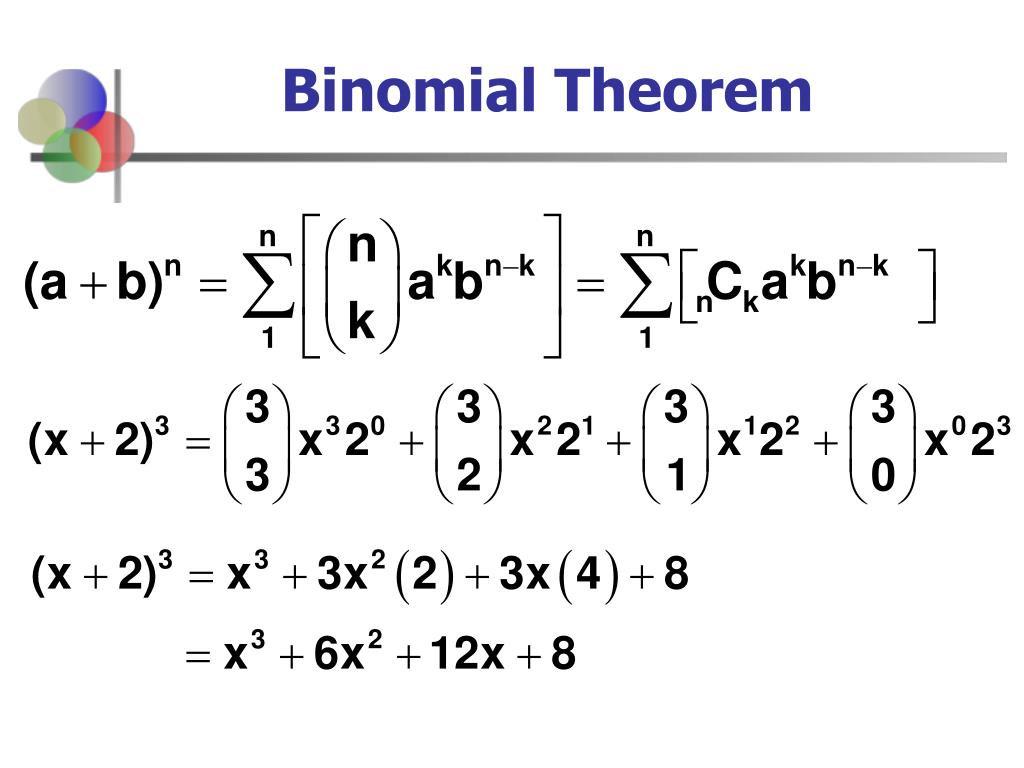 1024×768 binomial probability distribution powerpoint from www.slideserve.com
 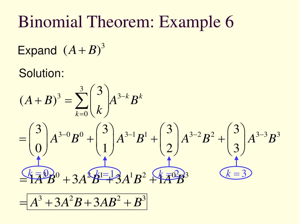 474×355 binomial theorem powerpoint id from www.slideserve.com
 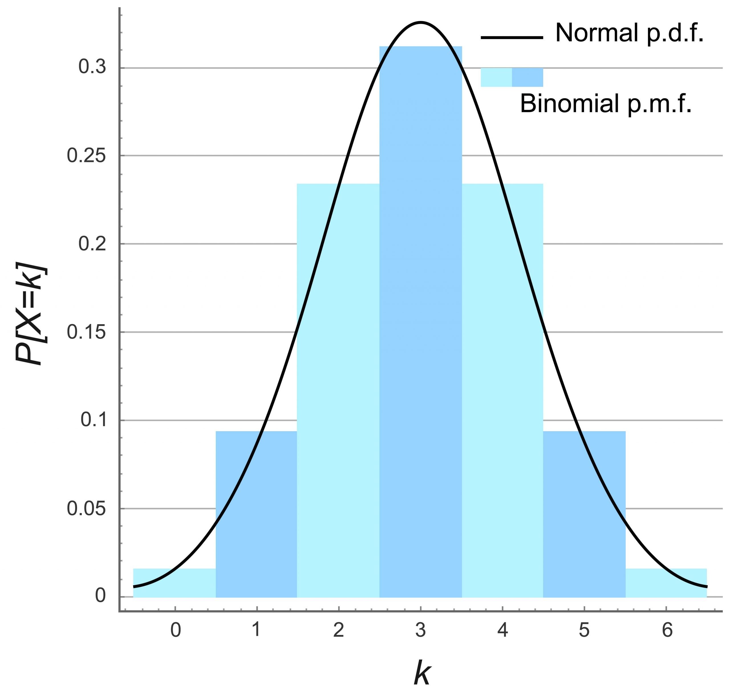 2560×2443 binomial probability distribution data science learning keystone from datasciencelk.com
  1280×720 binomial series expand function surefire examples from calcworkshop.com
  1800×900 binomial theorem explanation examples from www.storyofmathematics.com
  0 x 0 binomial distribution fully explained examples from calcworkshop.com
 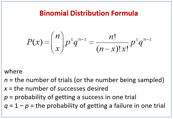 584×403 binomial distribution examples solutions formulas from www.onlinemathlearning.com
  1024×461 binomial distribution definition probability calculate negative from www.wallstreetmojo.com
  507×352 binomial series examples solutions from www.onlinemathlearning.com
  1024×768 binomial distribution powerpoint from www.slideserve.com
  406×185 binomial definition illustrated mathematics dictionary from www.mathsisfun.com
  1200×600 binomial theorem definition formula proof examples from www.adda247.com
  625×407 binomial distribution definition properties calculation formula from www.cuemath.com
  674×274 finding terms binomial expansion examples solutions worksheets from www.onlinemathlearning.com
  2560×1920 binomial coefficient from aussiemathematician.io
  1024×561 definition binomial math definitions letter from www.subjectcoach.com
  1000×500 binomial distribution business statistics definition formula from www.geeksforgeeks.org
  441×215 binomial theorem study material iit jee askiitians from www.askiitians.com
  1024×577 binomial expansion examples solutions agnes hendricks blog from storage.googleapis.com
  561×361 binomial theorem geeksforgeeks from www.geeksforgeeks.org
  700×412 binomial definition binomial from www.worksheetsplanet.com
  740×266 binomial theorem examples solutions examples worksheets from www.onlinemathlearning.com
  1280×720 binomial distribution youtube from www.youtube.com
  1000×600 binomial theorem proof math village from mathvilage.blogspot.com
  1513×877 binomial distribution quality gurus from www.qualitygurus.com
  750×356 binomial expansion formula examples solutions worksheets from www.onlinemathlearning.com
  600×280 phys binomial theorem from www.physics.udel.edu
  1024×526 binomial distribution formula calculator excel template from www.educba.com
  1024×768 binomial theorem from studylib.net
  1920×1080 lesson video binomial theorem nagwa from www.nagwa.com
  0 x 0 prove binomial theorem induction youtube from www.youtube.com
  1536×864 binomial nomenclature definition examples biology dictionary from www.biologyonline.com
  930×390 binomial expansion cie math solutions from ciemathsolutions.blogspot.com
  436×470 distribucion binomial formula ejemplos from elprofe.online
 :max_bytes(150000):strip_icc()/dotdash_v3_Understanding_the_Binomial_Option_Pricing_Model_Nov_2020-05-db5a8f5280ef404b8e2411bd063beef9.jpg) 6009×3959 understanding binomial option pricing model from www.investopedia.com
6009×3959 understanding binomial option pricing model from www.investopedia.com  1049×571 definition binomial nomenclature rules examples from www.ahmadcoaching.com
  1024×572 binomial theorem expand binomial express result from www.numerade.com
  1024×974 understanding shape binomial distribution from www.statology.org
  750×511 general middle terms binomial expansion formulas examples from byjus.com
  1640×1087 read binomial distribution table from www.statology.org
  1280×1920 demystifying binomial distribution dennis robert from towardsdatascience.com
  1024×630 overview binomial nomenclature rules from eduinput.com
  750×618 binomial nomenclature rules binomial nomenclature from byjus.com
  1665×551 binomial theorem studypug from www.studypug.com
  773×247 binomial expansion cureece from cureece.blogspot.com
  1024×768 binomial distribution examples dbinom pbinom qbinom rbinom from statisticsglobe.com
  1747×914 binomial theorem formula formula maths from formulainmaths.in
  1024×646 binomial theorem toppers bulletin from www.toppersbulletin.com
  1024×768 binomial probability formula statistics theprobability from theprobability.netlify.app
